solutions_tutorial01

Tutorial 1: Inferring phylogenies using maximum likelihood

In this tutorial you will be guided in using PhyML and its extension, CodonPhyML, to solve common phylogenetic problems. For some of the following exercises there might be more than one single solution.

These exercises were prepared by Maria Anisimova

ML with DNA data (the primate DNA dataset)

Dataset file: primates-nt.phy

Exercise 1

GOAL: In this exercise you are asked to run PhyML twice in order to compare the effect of estimating nucleotide frequencies from the used dataset vs. optimising them with a maximum likelihood (ML) approach.

Execution

1. First run

Nucleotide substitution model = HKY85 + Gamma
Estimating transition/transversion ratio ( $\kappa$ parameter of HKY85 model)
Estimating alpha parameter (remember $\alpha = \beta$ for gamma distributions used in phylogenetics)
Estimating nucleotide frequencies with ML

Here is the list of the parameters to change:

From 2^nd menu

[M] ................. Model of nucleotide substitution  HKY85
[F] ................. Optimise equilibrium frequencies  yes
[T] .................... Ts/tv ratio (fixed/estimated)  estimated
[C] ........... Number of substitution rate categories  4
[G] ............. Gamma distributed rates across sites  yes
[A] ... Gamma distribution parameter (fixed/estimated)  estimated

2. Second run

Nucleotide substitution model = HKY85 + Gamma
Estimating transition/transversion ratio ( $\kappa$ parameter of HKY85 model)
Estimating alpha parameter (remember $\alpha = \beta$ for gamma distributions used in phylogenetics)
Estimating nucleotide frequencies empirically from the data

Here is the list of the parameters to change:

From 2^nd menu

[M] ................. Model of nucleotide substitution  HKY85
[F] ................. Optimise equilibrium frequencies  no
[T] .................... Ts/tv ratio (fixed/estimated)  estimated
[C] ........... Number of substitution rate categories  4
[G] ............. Gamma distributed rates across sites  yes
[A] ... Gamma distribution parameter (fixed/estimated)  estimated

Questions

1. Do you see much difference in the tree?

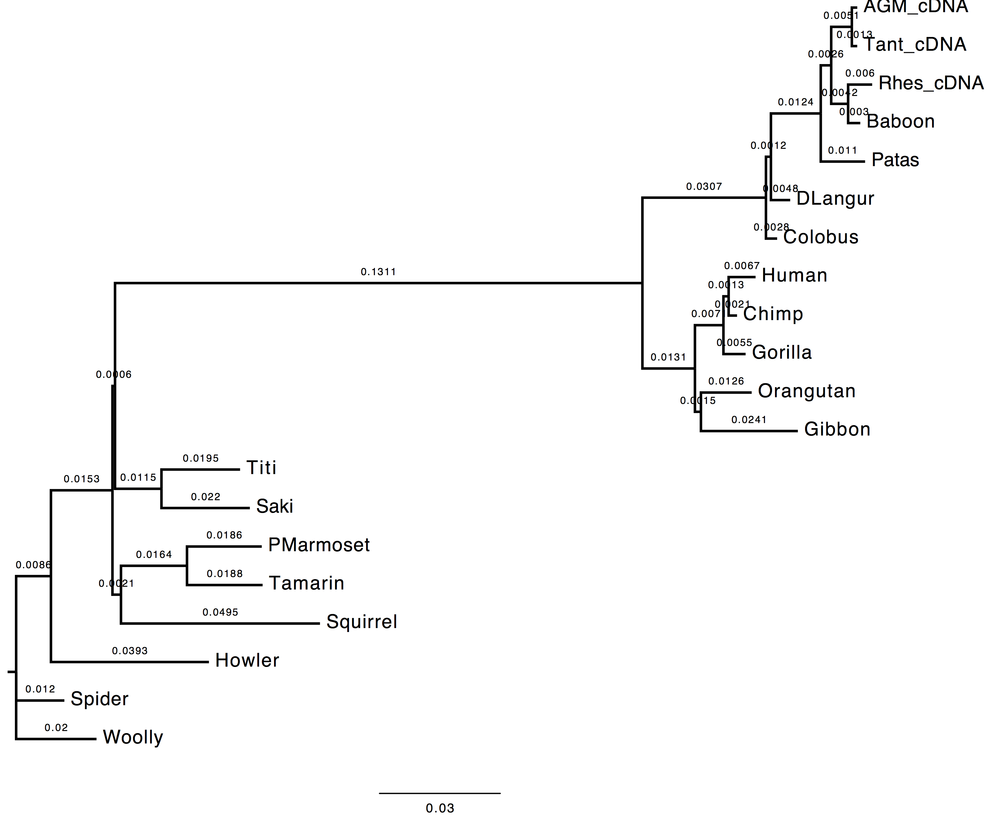
The topology does not change, however we can observe a change in the computed branch lengths.

Nt-frequencies optimised	Nt-frequencies estimated

2. In the likelihood value (stat file)?

The likelihood value of the tree inferred using the nucleotide frequencies estimated empirically from the dataset is lower than the likelihood value of the tree inferred using the nucleotide frequencies estimated via ML. This is due to dataset dimensions (the number of the sequences used).

    run 1: -6172.58045
    run 2: -6173.49655

3. Which option is best and why do you think so?

The best option in this case is to use the ML approach since the ML optimisation technique provides better estimates for the nucleotide frequencies, which, in turn, affect the likelihood of the inferred tree. This is due to the nucleotide frequencies which are used in the calculation of the likelihood of each site of the alignment ( $\pi Q = 0$ , where $\pi$ is the vector of the nucleotide frequencies and $Q$ the rate matrix).

Exercise 2

GOAL: In this exercise you are asked to optimise the tree topology on the substitution parameters obtained using ML performing a tree search (i.e. NNI, SPR, TBR) on the initial tree topology.

Execution

1. Run

Nucleotide substitution model = HKY85 + Gamma
Estimating transition/transversion ratio ( $\kappa$ parameter of HKY85 model)
Estimating alpha parameter (remember $\alpha = \beta$ for gamma distributions used in phylogenetics)
Estimating nucleotide frequencies with ML
No tree search (tree optimisation)

Here is the list of the parameters to change from the PhyML menu:

From 2^nd menu

[M] ................. Model of nucleotide substitution  HKY85
[F] ................. Optimise equilibrium frequencies  yes
[T] .................... Ts/tv ratio (fixed/estimated)  estimated
[C] ........... Number of substitution rate categories  4
[G] ............. Gamma distributed rates across sites  yes
[A] ... Gamma distribution parameter (fixed/estimated)  estimated

From 3^rd menu

[O] ........................... Optimise tree topoLOGy  no

Questions

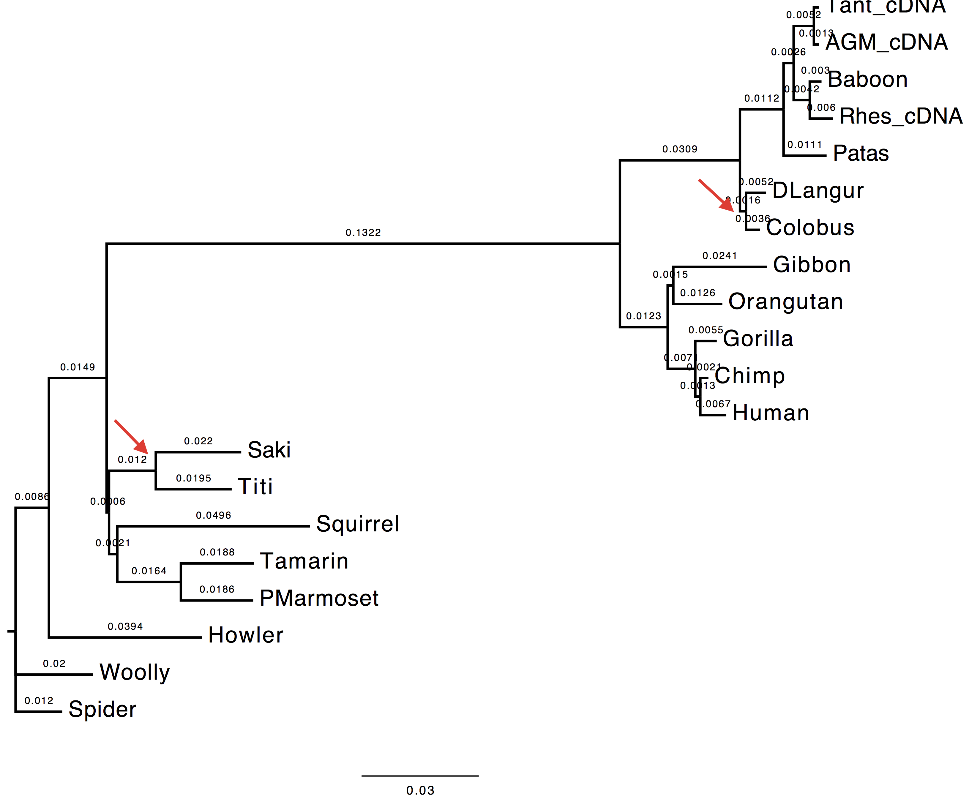
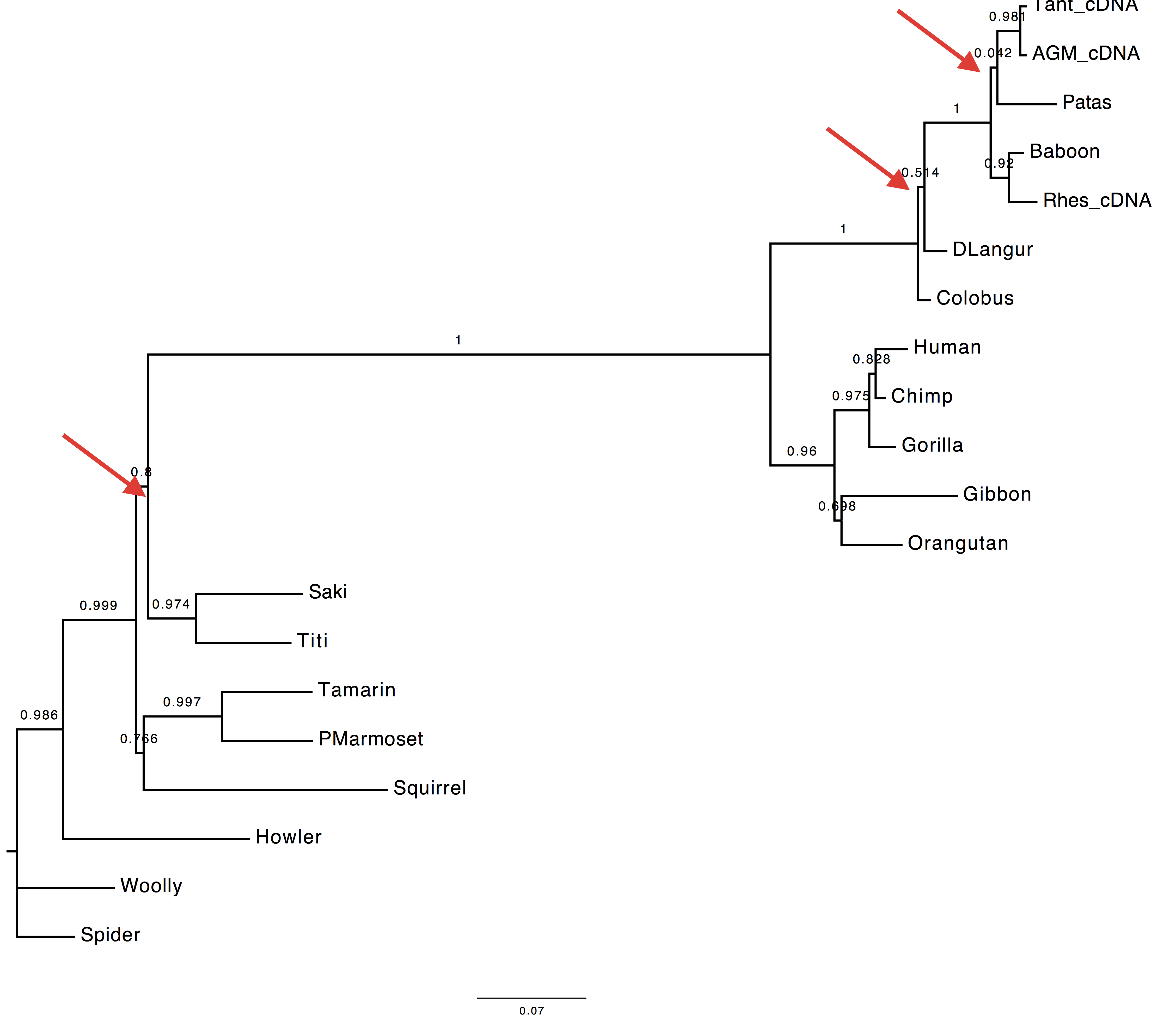
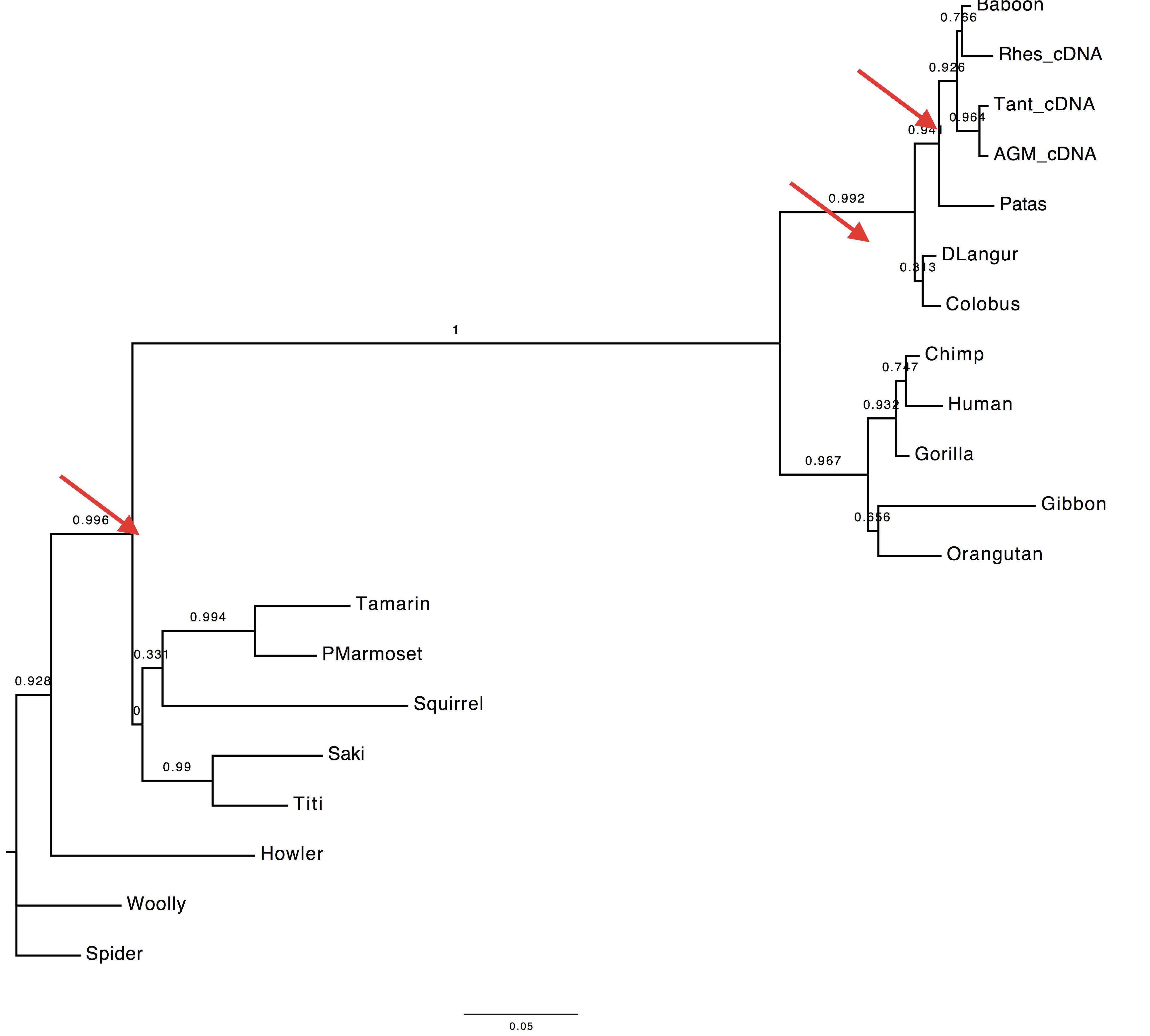
1. Compare the trees obtained with and without tree-search. What do you observe and why?

The topology inferred without tree search presents a variation in the internal node attribution for the clades (DLangur, Colobus) and (Saki,Titi).

With tree-search	Without tree-search

2. Compare the model estimates with and without tree-search. What do you observe and why?

The transition/transversion ratio differs slightly between the two runs. As the matter of fact, $k$ parameter appears to have a higher value when tree-search is not performed.

3. Compare the likelihood of the ML and NJ trees. What do you observe and why?

The likelihood value obtained without tree-search is lower than the value obtain performing the topology optimisation. This value is expected since the substitution parameters are optimised over the first inferred tree topology which did not undergo any refinement.

    with tree-search: -6172.58045
    without tree-search: -6173.00555

Exercise 3

GOAL: In this exercise you are asked to compare different substitution models (and their variations) on the same dataset.

Execution

Model	Log-likelihood	Parameters	AIC
JC	-6379.66383	38	12835.32766
JC_I	-6311.41650	39	12700.833
JC_G	-6304.38084	39	12686.76168
JC_G_I	-6304.35263	40	12688.70526
HKY	-6251.43051	42	12586.86102
HKY_I	-6180.09689	43	12446.19378
HKY_G	-6172.58045	43	12431.1609
HKY_G_I	-6172.52896	44	12433.05792
GTR	-6241.48788	46	12574.97576
GTR_I	-6171.17472	47	12436.34944
GTR_G	-6163.87291	47	12421.74582
GTR_G_I	-6172.52896	48	12441.05792

The number of parameters are computed in the following way for a rooted
tree:

$k = (2 \ast \text{no. taxa} - 2) + \text{no. parameters in substitution model} + \text{extra parameters}$

substitution models: JC = 0 parameters | HKY = 4 parameters | GTR = 8
parameters
invariant sites = +1 parameter
gamma rates = +1 parameter

We compute the AIC value as follows:

$AIC = 2(k) - \log(L)$

Questions

1. Which model is the best (including HKY+Gamma), based on the AIC criterion?

We select the model with the lowest AIC value. In this case, GTR + Gamma

This exercise can also be solved using jmodeltest which performs automatically phylogenetic tree reconstructions with every model and extra parameters (i.e. invariant sites, gamma).

Exercise 4

GOAL: In this exercise you are asked to compute the branch support using different statistical methods. We are going to evaluate it on the phylogenetic tree evaluated with the following settings:

    . Tree topology search :        NNIs
    . Initial tree:                 BioNJ
    . Model of nucleotides substitution:    GTR
    . Number of taxa:           20
    . Log-likelihood:           -6163.87291
    . Unconstrained likelihood: -5060.29926
    . Parsimony:                741
    . Tree size:                0.54568
    . Discrete gamma model:     Yes
      - Number of categories:           4
      - Gamma shape parameter:      0.565
    . Nucleotides frequencies:
      - f(A)= 0.29130
      - f(C)= 0.21021
      - f(G)= 0.25260
      - f(T)= 0.24589
    . GTR relative rate parameters : 
      A <-> C    1.62195
      A <-> G    4.11843
      A <-> T    0.80648
      C <-> G    1.47358
      C <-> T    3.64931
      G <-> T    1.00000

    . Instantaneous rate matrix : 
      [A---------C---------G---------T------]
      -1.00085   0.21604   0.65916   0.12565  
       0.29937  -1.10379   0.23585   0.56858  
       0.76015   0.19627  -1.11222   0.15580  
       0.14885   0.48607   0.16005  -0.79498

Execution

We are going to run PhyML twice: once using the non parametric bootstrap and the second time using the SH-aLRT method.

1. First run

[B] ................ Non parametric bootstrap analysis  yes (100 replicates)
[A] ................ Approximate likelihood ratio test  no

We perform a bootstrap analysis using 100 replicates (4^th^ menu).

Bootstrap analysis assumes that:
- sites are independently and identically distributed (i.i.d.)
- Amplifies the biases of the tree inference method
- Often conservative (>70% is considered strong support, but no guarantee)
- Slow for large datasets
- Difficult to interpret

2. Second run

  [B] ................ Non parametric bootstrap analysis  no
  [A] ................ Approximate likelihood ratio test  yes / aLRT statistics

We perform an sh-aLRT analysis (4^th^ menu).

SH-aLRT method assumes that:
- the branch being studied provides a significant likelihood gain.
- per each branch two alternative hypotheses are tested: a null hypothesis where the branch is collapsed and the rest of the topology is maintained vs. an alternative hypothesis where the branch length is kept and the topology is intact.
- aLRT is much faster than bootstrap

Questions

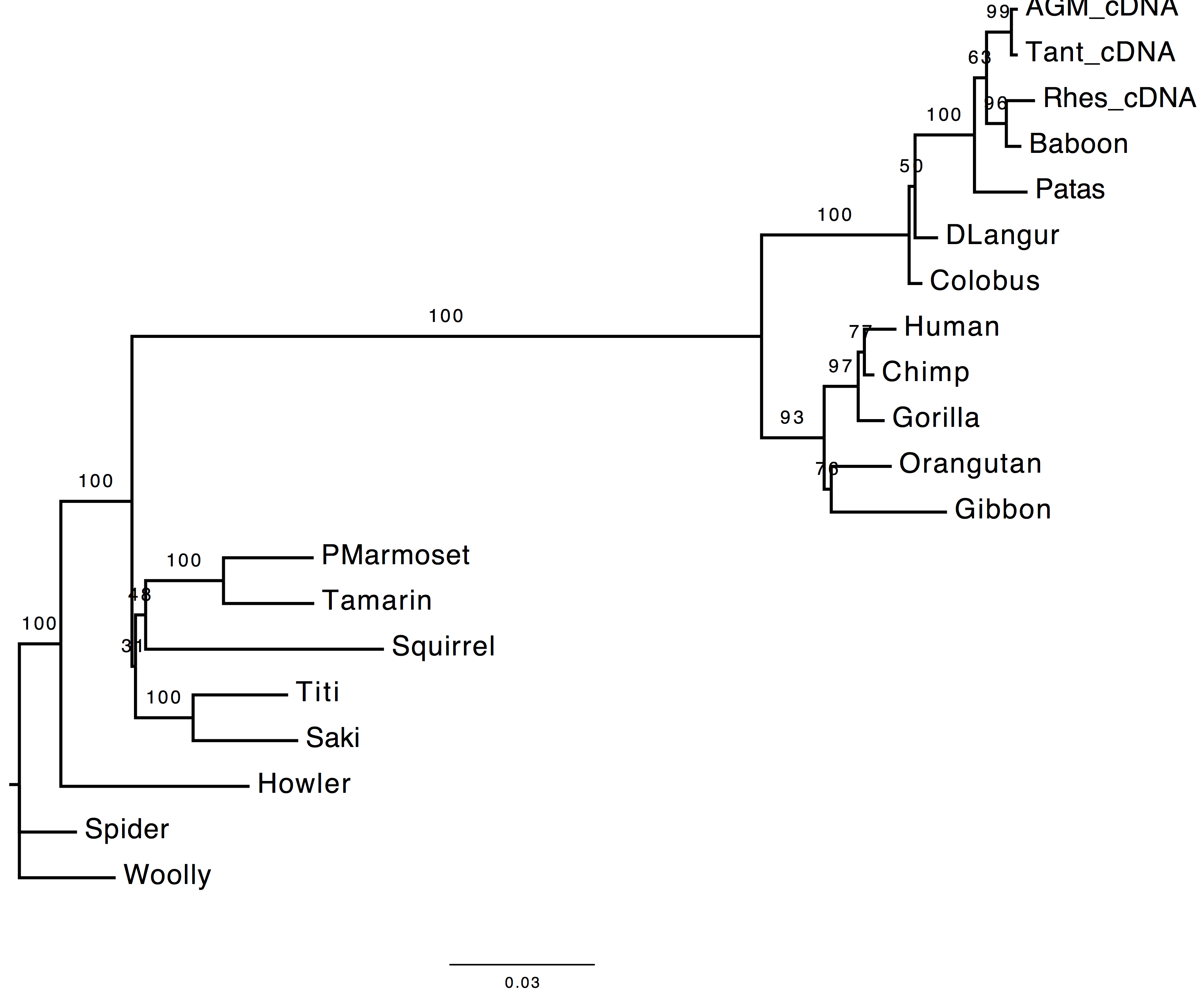
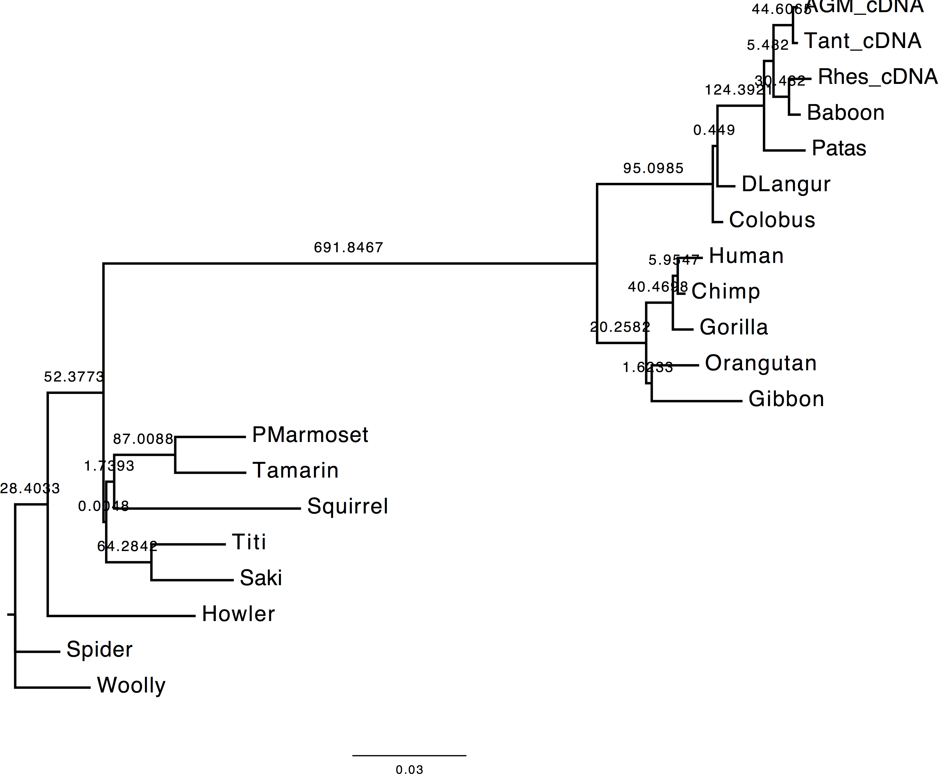
1. Are the results compatible?

Both the methods used to infer the branch support appear to agree on the support provided by long branches, however they do not agree for short ones. These two methods infer branch support using completely different strategies.

With bootstrap support	With sh-aLRT support

Exercise 5

For linux/Mac Os X

We assume PhyML binary is included in the user PATH variable and it can be called with phyml

Positioning in the directory containing the dataset:

cd path/to/tutorial01_phyml

ex. 1

run1> phyml -i primates-nt.phy -m 'HKY85' -t 'e' -a 'e'  f 'm'
run2> phyml -i primates-nt.phy -m 'HKY85' -t 'e' -a 'e' -f 'e'

ex. 2

run1> phyml -i primates-nt.phy -m 'HKY85' -t 'e' -a 'e' -f 'm' -o 'lr'

ex. 3

JC      > phyml -i primates-nt.phy -m 'JC69' -t 'e' -a 'e' -f 'm' -c 1
JC_I    > phyml -i primates-nt.phy -m 'JC69' -t 'e' -a 'e' -f 'm' -c 1 -v 'e'
JC_G    > phyml -i primates-nt.phy -m 'JC69' -t 'e' -a 'e' -f 'm'
JC_I_G  > phyml -i primates-nt.phy -m 'JC69' -t 'e' -a 'e' -f 'm' -v 'e'

HKY     > phyml -i primates-nt.phy -m 'HKY85' -t 'e' -a 'e' -f 'm' -c 1
HKY_I   > phyml -i primates-nt.phy -m 'HKY85' -t 'e' -a 'e' -f 'm' -c 1 -v 'e'
HKY_G   > phyml -i primates-nt.phy -m 'HKY85' -t 'e' -a 'e' -f 'm'
HKY_I_G > phyml -i primates-nt.phy -m 'HKY85' -t 'e' -a 'e' -f 'm' -v 'e'

GTR     > phyml -i primates-nt.phy -m 'GTR' -t 'e' -a 'e' -f 'm' -c 1
GTR_I   > phyml -i primates-nt.phy -m 'GTR' -t 'e' -a 'e' -f 'm' -c 1 -v 'e'
GTR_G   > phyml -i primates-nt.phy -m 'GTR' -t 'e' -a 'e' -f 'm'
GTR_I_G > phyml -i primates-nt.phy -m 'GTR' -t 'e' -a 'e' -f 'm' -v 'e'

ex. 4

Bootstrap(100) > phyml -i primates-nt.phy -m 'HKY85' -t 'e' -a 'e' -f 'e' -b 100
SH-aLRT        > phyml -i primates-nt.phy -m 'HKY85' -t 'e' -a 'e' -f 'e' -b -4

Exercise 6

GOAL:

Execution

Preprocessing

The dataset should not include any stop codon, therefore we modify the dataset deleting the last 3 columns (the last codon) from the MSA. In order to do so, you can open primates-nt.phy with AliView and after selecting the last 3 columns press delete on the keyboard. Save the new file as Phylip with the following name primates-nt-nostop.phy.

For models M0, M0+Gamma and M5

From 1^st menu

[D] ................. Data type (DNA/AA/CODON/Generic)  CODON
[E] ............................... Matrix exponential  eigenvalues
[H] ... Optimization heuristic for tree reconstruction  original
[O] .................. Parameter optimization strategy  multivariate (BFGS)
[I] ...... Input sequences interleaved (or sequential)  interleaved
[M] ....................... Analyze multiple data sets  no

From 2^nd menu

[m] ...... Model type (parametric/empirical/semi-emp.)  parametric
[M] ...................... Model of codon substitution  GY
[i] ..... Initial pairwise distances using codon model  KOSI07
[g] ..................................... Genetic code  Standard
[W] ................. Model for Dn/Ds ratio (M0/M3/M5)  M0
[P] ...................... Equilibrium frequency model  CF3x4
[F] ............................ Origin of frequencies  ML estim.
[T] .................... Ts/Tv ratio (fixed/estimated)  estimated
[D] .................... Dn/Ds ratio (fixed/estimated)  estimated
[V] . Proportion of invariable sites (fixed/estimated)  fixed (p-invar = 0.00)
[R] ....... One category of substitution rate (yes/no)  yes

M0+Gamma

From 2^nd menu

[m] ...... Model type (parametric/empirical/semi-emp.)  parametric
[M] ...................... Model of codon substitution  GY
[i] ..... Initial pairwise distances using codon model  KOSI07
[g] ..................................... Genetic code  Standard
[W] ................. Model for Dn/Ds ratio (M0/M3/M5)  M0
[P] ...................... Equilibrium frequency model  CF3x4
[F] ............................ Origin of frequencies  ML estim.
[T] .................... Ts/Tv ratio (fixed/estimated)  estimated
[D] .................... Dn/Ds ratio (fixed/estimated)  estimated
[V] . Proportion of invariable sites (fixed/estimated)  fixed (p-invar = 0.00)
[R] ....... One category of substitution rate (yes/no)  no
[C] ........... Number of substitution rate categories  4
[A] ... Gamma distribution parameter (fixed/estimated)  estimated
[G] .........'Middle' of each rate class (mean/median)  mean

[m] ...... Model type (parametric/empirical/semi-emp.)  parametric
[M] ...................... Model of codon substitution  GY
[i] ..... Initial pairwise distances using codon model  KOSI07
[g] ..................................... Genetic code  Standard
[W] ................. Model for Dn/Ds ratio (M0/M3/M5)  M5
[w] ................. Number of Dn/Ds ratio categories  3
[P] ...................... Equilibrium frequency model  CF3x4
[F] ............................ Origin of frequencies  ML estim.
[T] .................... Ts/Tv ratio (fixed/estimated)  estimated
[D] .................... Dn/Ds ratio (fixed/estimated)  gamma distribution
[a] .. Gamma distribution alpha/beta (fixed/estimated)  estimated
[G] .........'Middle' of each rate class (mean/median)  mean
[V] . Proportion of invariable sites (fixed/estimated)  fixed (p-invar = 0.00)

For models LG, WAG, LG+Gamma and WAG+Gamma

[D] ................. Data type (DNA/AA/CODON/Generic)  AA
[d] ............. Convert NT sequence into AA sequence  yes
[G] ..................................... Genetic code  Standard
[I] ...... Input sequences interleaved (or sequential)  interleaved
[M] ....................... Analyze multiple data sets  no

[M] ................ Model of amino-acids substitution  LG
[F] .. Amino acid frequencies (model/empiric/optimize)  model
[V] . Proportion of invariable sites (fixed/estimated)  fixed (p-invar = 0.00)
[R] ....... One category of substitution rate (yes/no)  yes

WAG

[M] ................ Model of amino-acids substitution  WAG
[F] .. Amino acid frequencies (model/empiric/optimize)  model
[V] . Proportion of invariable sites (fixed/estimated)  fixed (p-invar = 0.00)
[R] ....... One category of substitution rate (yes/no)  yes

LG+Gamma

[M] ................ Model of amino-acids substitution  LG
[F] .. Amino acid frequencies (model/empiric/optimize)  model
[V] . Proportion of invariable sites (fixed/estimated)  fixed (p-invar = 0.00)
[R] ....... One category of substitution rate (yes/no)  no
[C] ........... Number of substitution rate categories  4
[A] ... Gamma distribution parameter (fixed/estimated)  estimated
[G] .........'Middle' of each rate class (mean/median)  mean

WAG+Gamma

[M] ................ Model of amino-acids substitution  WAG
[F] .. Amino acid frequencies (model/empiric/optimize)  model
[V] . Proportion of invariable sites (fixed/estimated)  fixed (p-invar = 0.00)
[R] ....... One category of substitution rate (yes/no)  no
[C] ........... Number of substitution rate categories  4
[A] ... Gamma distribution parameter (fixed/estimated)  estimated
[G] .........'Middle' of each rate class (mean/median)  mean

GTR+Gamma

From 1^st menu

[D] ................. Data type (DNA/AA/CODON/Generic)  DNA
[I] ...... Input sequences interleaved (or sequential)  interleaved
[M] ....................... Analyze multiple data sets  no

From 2^nd menu

[M] ................. Model of nucleotide substitution  GTR
[F] ................. Optimise equilibrium frequencies  yes
[V] . Proportion of invariable sites (fixed/estimated)  fixed (p-invar = 0.00)
[R] ....... One category of substitution rate (yes/no)  no
[C] ........... Number of substitution rate categories  4
[A] ... Gamma distribution parameter (fixed/estimated)  estimated
[G] .........'Middle' of each rate class (mean/median)  mean

The number of parameters are computed in the following way for a rooted tree:

$k = (2 \ast \text{no. taxa} - 2) + \text{no. parameters in substitution model} + \text{extra parameters}$
substitution models: LG = 0 parameters | WAG = 0 parameters | GTR = 8
parameters | GY = 2 | M0 = 2 | M5 = 2
gamma rates = +1 parameter

We compute the AIC value as follows:

$AIC = 2(k) - \log(L)$

Model	Log-likelihood	Parameters	AIC
GTR_G	-6158.95	47	12411.90
LG	-4826.14	38	9728.28
LG_G	-4735.17	39	9548.34
M0	-6163.53	40	12407.06
M0_G	-6075.69	41	12233.38
M5	-6057.39	40	12194.78
WAG	-4785.42	38	9646.84
WAG_G	-4702.97	39	9483.94

Questions

1. Based on AIC, which model fits your dataset best?

WAG + Gamma

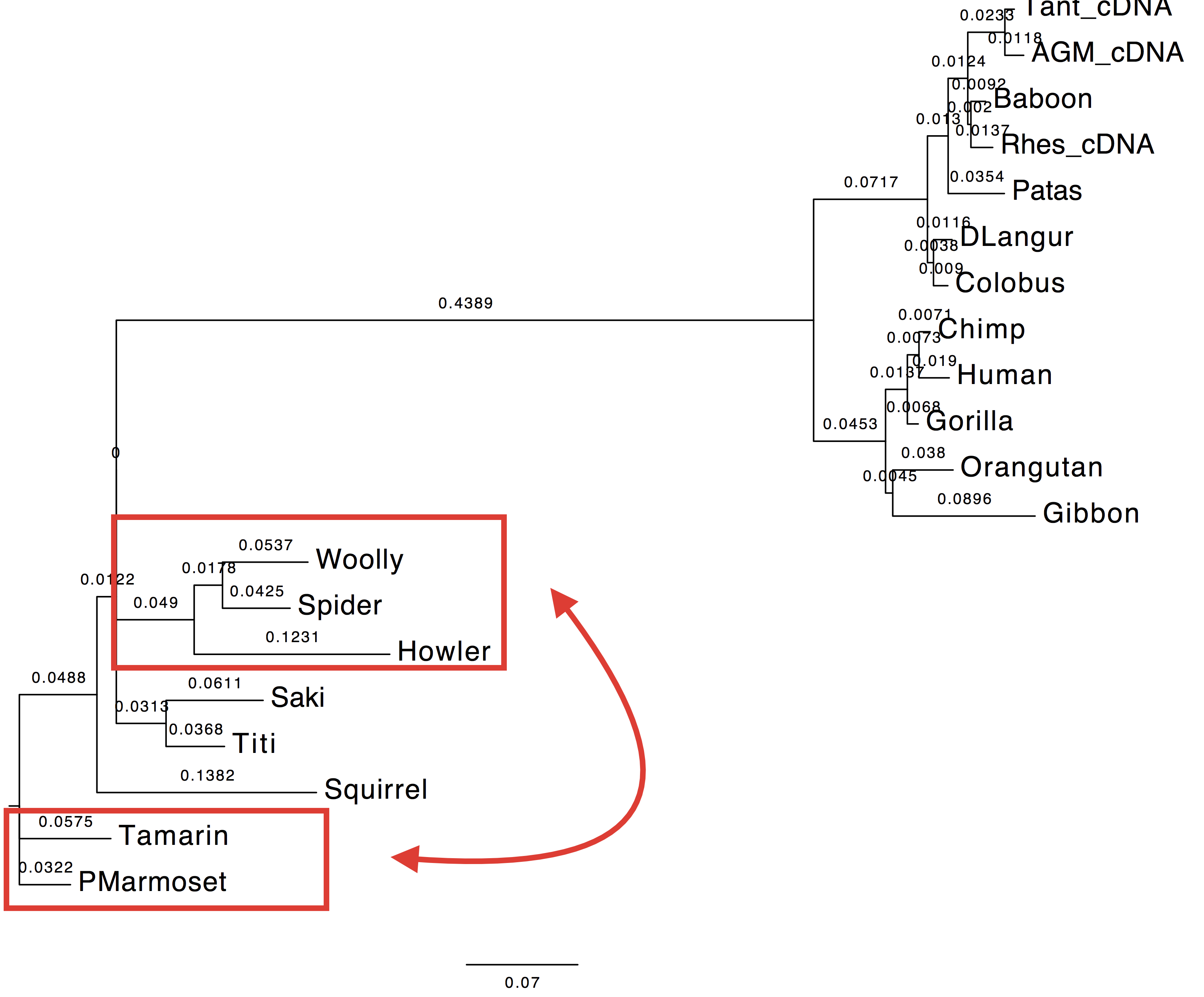
2. Are the trees inferred using the best AA and best codon model different?

According to the AIC ranking, the best codon model should be M5.

Herewith the two trees.

Using codon model	Using AA model

3. Are they different to the tree inferred using the DNA model?
Yes, they are also different to the tree inferred using the GTR+Gamma model.

ML with protein data

With primate dataset

GOAL: Testing different amino acids substitution models on a protein dataset

Dataset: primates-aa.phy

Execution

1. Using PhyML

We performed the analyses using PhyML and combining the following
settings accordingly to the requests:

[M] ................ Model of amino-acids substitution  LG
[F] . Amino acid frequencies (empirical/model defined)  model
[V] . Proportion of invariable sites (fixed/estimated)  fixed (p-invar = 0.00)
[R] ....... One category of substitution rate (yes/no)  yes

From the analyses we retrieved:

Model	Log-likelihood	Parameters	AIC
LG_G	-5199.88631	39	10477.77262
LG_G_I	-5199.55701	40	10479.11402
LG_G_F	-5230.44821	58	10576.89642
LG_G_F_I	-5230.08104	59	10578.16208

2. Using ProtTest webservice

You can find the results in the file ex7/prottest_analysis.txt

Questions

1. Which is the best model based on AIC criterion? What about using invariant sites?

We selected the LG + Gamma model according to the AIC criterion. Using the invariant sites does not influence the model selection. Adding a proportion of invariant sites increases the number of parameters, therefore the AIC penalises the inferred log-likelihood value.

2. Compare the trees, likelihood and AIC values to those of LG+Gamma.

Value	Tree estimated with LG+Gamma	Tree estimated with HIVw+G+F
Log-Likelihood:	-5199.89	-5013.50
AIC:	10477.77	10141.01
Tree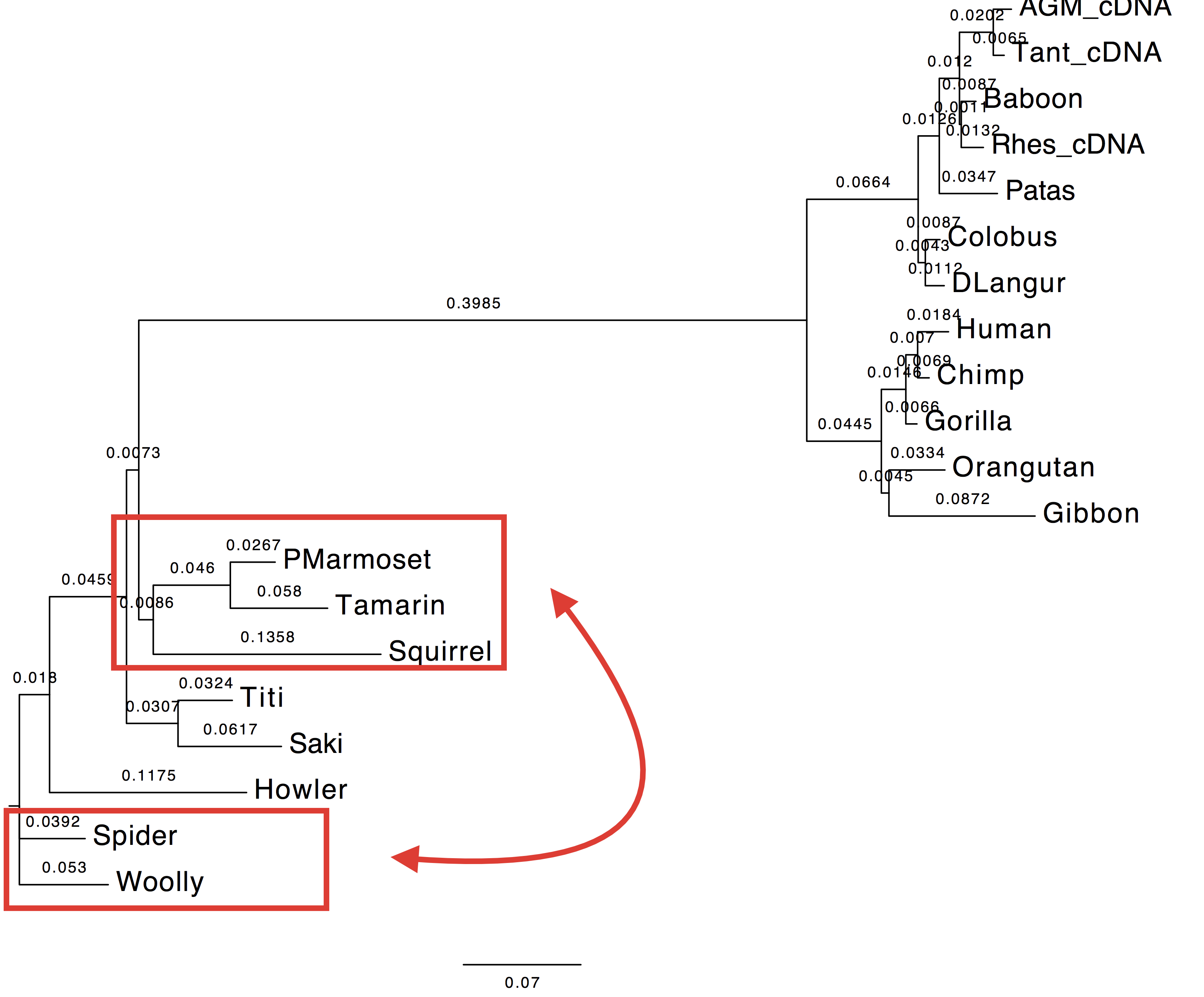

With protein data sets from Lerat et al. (2003)

GOAL: Inferring a phylogenetic tree on a protein dataset using an appropriate substitution model and detect an event of HGT.

Execution

1. Using PhyML

We used a selection of candidate substitution models (JTT, LG, WAG) that are suitable for the protein datasets.

dataset: Prot_biob.phy

Model	Log-likelihood	Parameters	AIC
JTT_G_I	-4593.61928	40	9267.23856
LG_G_I	-4546.51747	40	9173.03494
WAG_G_I	-4564.41245	40	9208.8249

We ranked the tested models according to the AIC statistics and we selected the LG+G+I model which best fits our dataset.

2. Using ProtTest webservice

You can find the results in the file ex8/prottest_analysis.txt

The best model in output from the model selection analysis is WAG+G+F

Questions

1. What can you tell based on the ML estimates?

Parameter	Using LG+G+I model	Using WAG+G+F model
Log-likelihood:	-4546.52	-4542.71
Gamma shape parameter:	0.953	0.633
Proportion of invariant:	0.182	0

When LG+G+I model is used, the alpha parameter of the gamma distribution is skewed towards $\alpha = 1$ which in turns indicate that the rate variability is centred on one category.

2. Display trees

We coloured the branches according to their support (blue = 1, red=0).

Using LG+G+I model	Using WAG+G+F model

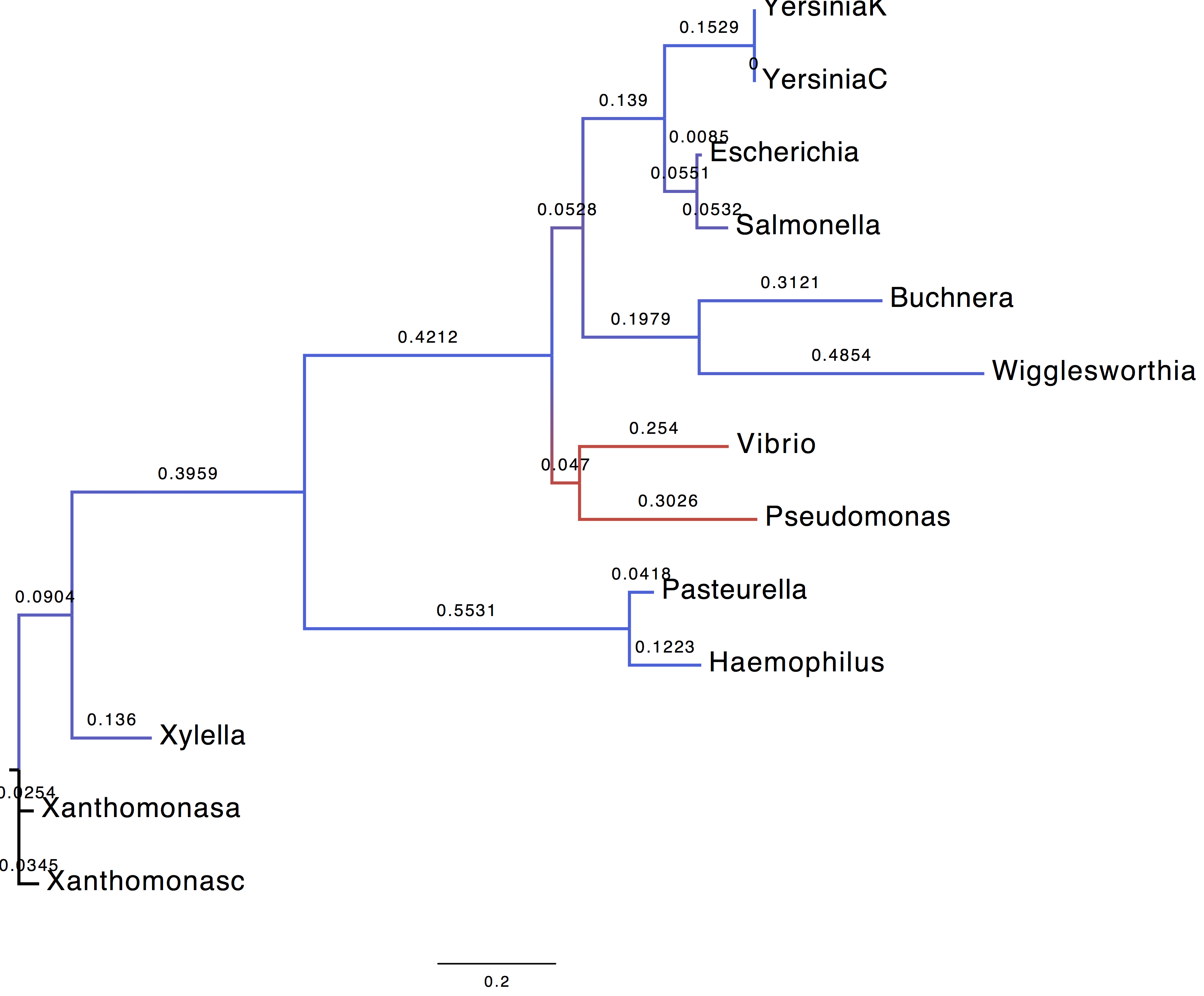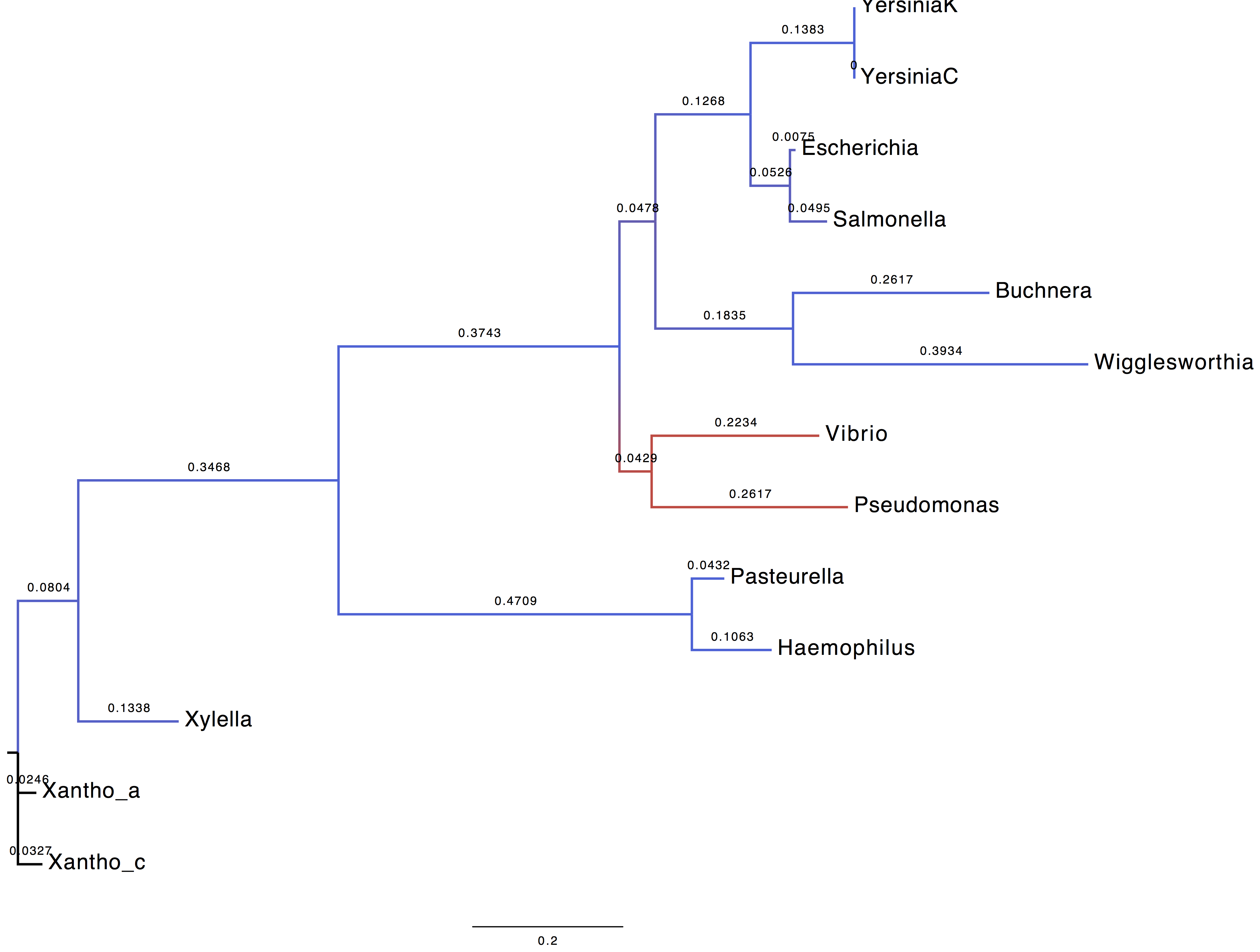3. Are you able to recover the HGT (horizontal gene transfer) published by Lerat et al.?

References

Darriba D, Taboada GL, Doallo R, Posada D. 2012. jModelTest 2: more models, new heuristics and parallel computing. Nature Methods 9(8), 772. http://dx.doi.org/10.1038/nmeth.2109
Guindon S and Gascuel O (2003). A simple, fast and accurate method to estimate large phylogenies by maximum-likelihood”. Systematic Biology 52:696-704. DOI:10.1080/10635150390235520
PhyML Manual
Lerat E, Daubin V, Moran NA (2003) From Gene Trees to Organismal Phylogeny in Prokaryotes:The Case of the γ-Proteobacteria. PLoS Biol 1(1): e19. doi: 10.1371/journal.pbio.000001

Document last updated on 02.02.2016

© 2016 Lorenzo Gatti – Applied Computational Genomic Team (ACGT) @
Institute of Applied Simulations (ZHAW) | Wädenswil | Zürich